%pylab inline
import scipy.signal as dsp
Populating the interactive namespace from numpy and matplotlib
Uncertainty propagation for IIR filters
from PyDynamic.misc.testsignals import rect
from PyDynamic.uncertainty.propagate_filter import IIRuncFilter
from PyDynamic.uncertainty.propagate_MonteCarlo import SMC
from PyDynamic.misc.tools import make_semiposdef
Digital filters with infinite impulse response (IIR) are a common tool in signal processing. Consider the measurand to be the output signal of an IIR filter with z-domain transfer function
The measurement model is thus given by
As input quantities to the model the input signal values \(x[k]\) and the IIR filter coefficients \((b_0,\ldots,a_{N_a})\) are considered.
Linearisation-based uncertainty propagation
Scientific publication
A. Link and C. Elster,
“Uncertainty evaluation for IIR filtering using a
state-space approach,”
Meas. Sci. Technol., vol. 20, no. 5, 2009.
The linearisation method for the propagation of uncertainties through the IIR model is based on a state-space model representation of the IIR filter equation
where
The linearization-based uncertainty propagation method for IIR filters provides
propagation schemes for white noise and colored noise in the filter input signal
incorporation of uncertainties in the IIR filter coefficients
online evaluation of the point-wise uncertainties associated with the IIR filter output
Implementation in PyDynamic
y,Uy = IIRuncFilter(x,noise,b,a,Uab)
with
xthe filter input signal sequencynoisethe standard deviation of the measurement noise in xb,athe IIR filter coefficientUabthe covariance matrix associated with \((a_1,\ldots,b_{N_b})\)
Remark
Implementation for more general noise processes than white noise is considered for one of the next revisions.
Example
# parameters of simulated measurement
Fs = 100e3
Ts = 1.0/Fs

# nominal system parameter
fcut = 20e3
L = 6
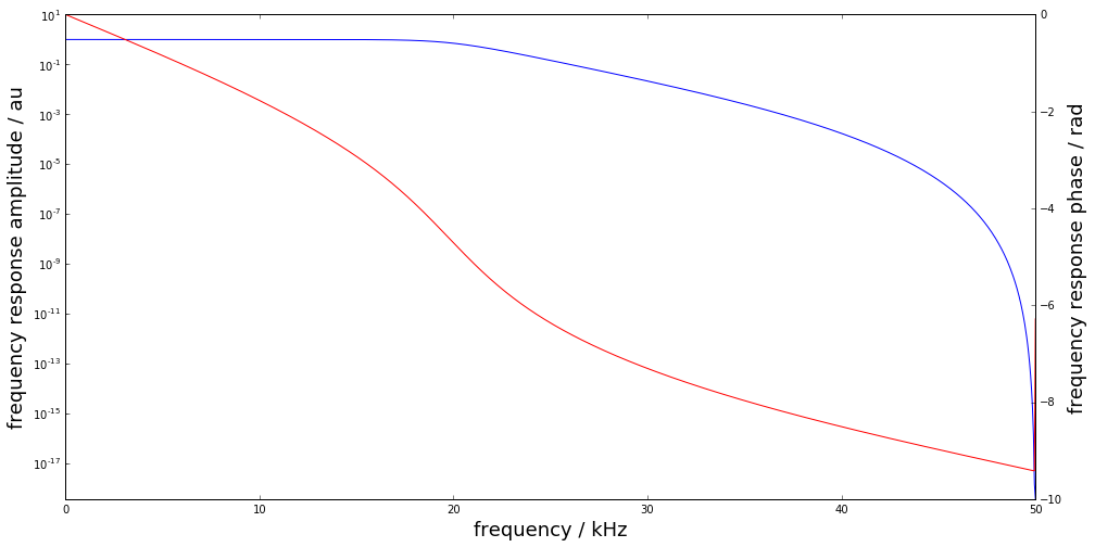
b,a = dsp.butter(L,2*fcut/Fs,btype='lowpass')
f = linspace(0,Fs/2,1000)
figure(figsize=(16,8))
semilogy(f*1e-3, abs(dsp.freqz(b,a,2*np.pi*f/Fs)[1]))
ylim(0,10);
xlabel("frequency / kHz",fontsize=18); ylabel("frequency response amplitude / au",fontsize=18)
ax2 = gca().twinx()
ax2.plot(f*1e-3, unwrap(angle(dsp.freqz(b,a,2*np.pi*f/Fs)[1])),color="r")
ax2.set_ylabel("frequency response phase / rad",fontsize=18);
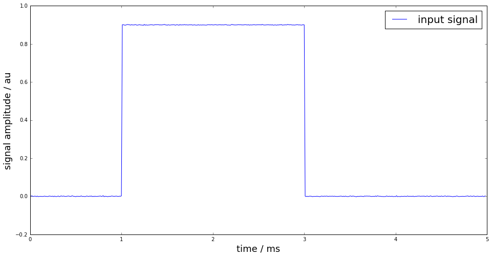
time = np.arange(0,499*Ts,Ts)
t0 = 100*Ts; t1 = 300*Ts
height = 0.9
noise = 1e-3
x = rect(time,t0,t1,height,noise=noise)
figure(figsize=(16,8))
plot(time*1e3, x, label="input signal")
legend(fontsize=20)
xlabel('time / ms',fontsize=18)
ylabel('signal amplitude / au',fontsize=18);
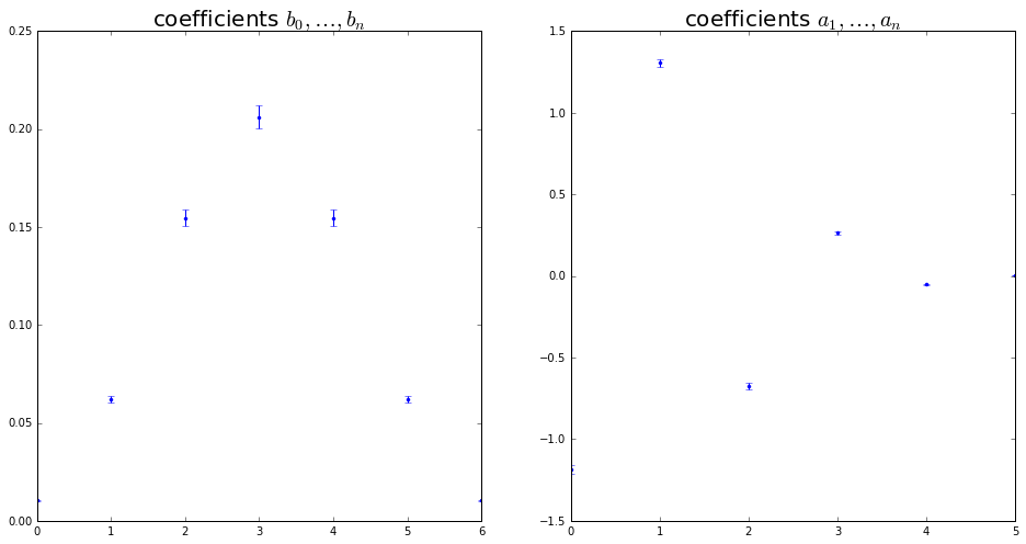
# uncertain knowledge: fcut between 19.8kHz and 20.2kHz
runs = 10000
FC = fcut + (2*np.random.rand(runs)-1)*0.2e3
AB = np.zeros((runs,len(b)+len(a)-1))

for k in range(runs):
    bb,aa = dsp.butter(L,2*FC[k]/Fs,btype='lowpass')
    AB[k,:] = np.hstack((aa[1:],bb))

Uab = make_semiposdef(np.cov(AB,rowvar=0))
Uncertain knowledge: low-pass cut-off frequency is between \(19.8\) and \(20.2\) kHz
figure(figsize=(16,8))
subplot(121)
errorbar(range(len(b)), b, sqrt(diag(Uab[L:,L:])),fmt=".")
title(r"coefficients $b_0,\ldots,b_n$",fontsize=20)
subplot(122)
errorbar(range(len(a)-1), a[1:], sqrt(diag(Uab[:L, :L])),fmt=".");
title(r"coefficients $a_1,\ldots,a_n$",fontsize=20);
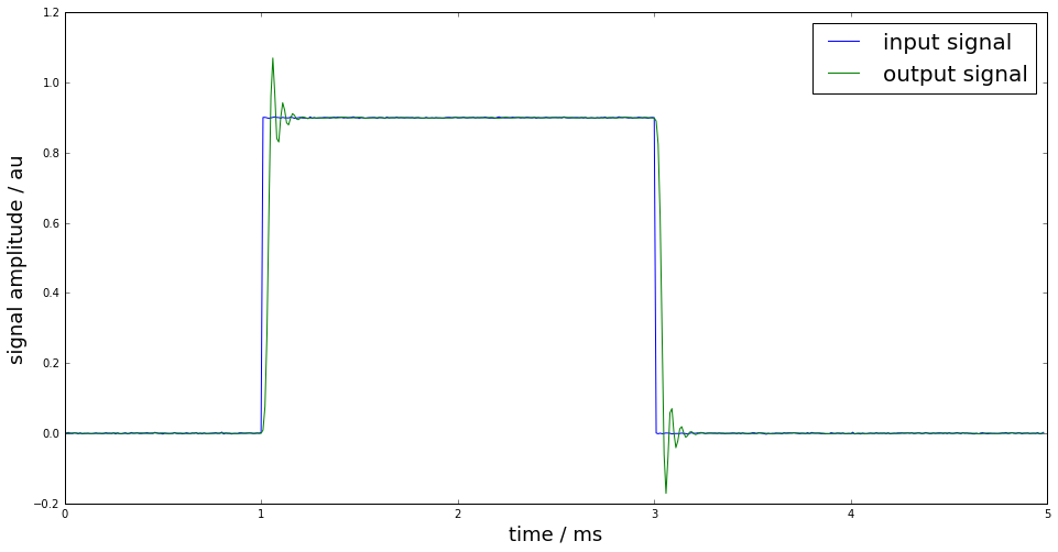
Estimate of the filter output signal and its associated uncertainty
y,Uy = IIRuncFilter(x,noise,b,a,Uab)

figure(figsize=(16,8))
plot(time*1e3, x, label="input signal")
plot(time*1e3, y, label="output signal")
legend(fontsize=20)
xlabel('time / ms',fontsize=18)
ylabel('signal amplitude / au',fontsize=18);
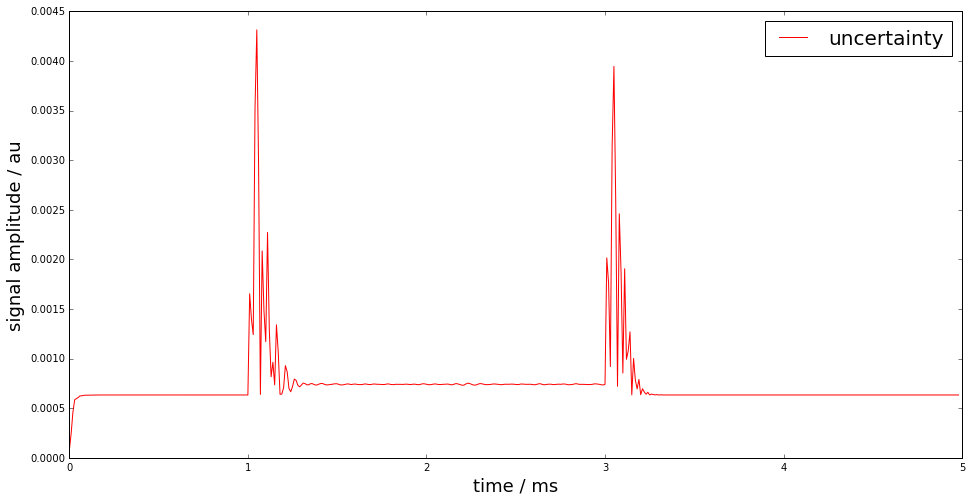
figure(figsize=(16,8))
plot(time*1e3, Uy, "r", label="uncertainty")
legend(fontsize=20)
xlabel('time / ms',fontsize=18)
ylabel('signal amplitude / au',fontsize=18);
Monte-Carlo method for uncertainty propagation
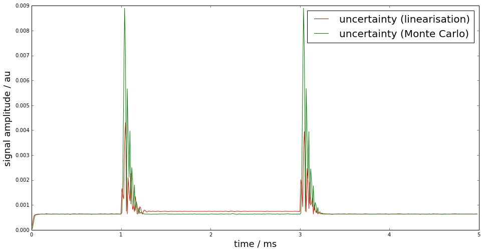
The linearisation-based uncertainty propagation can become unreliable due to the linearisation errors. Therefore, a Monte-Carlo method for digital filters with uncertain coefficients has been proposed in
S. Eichstädt, A. Link, P. Harris, and C. Elster,
“Efficient implementation of a Monte Carlo method
for uncertainty evaluation in dynamic measurements,”
Metrologia, vol. 49, no. 3, 2012.
The proposed Monte-Carlo method provides - a memory-efficient implementation of the GUM Monte-Carlo method - online calculation of point-wise uncertainties, estimates and coverage intervals by taking advantage of the sequential character of the filter equation
yMC,UyMC = SMC(x,noise,b,a,Uab,runs=10000)

figure(figsize=(16,8))
plot(time*1e3, Uy, "r", label="uncertainty (linearisation)")
plot(time*1e3, UyMC, "g", label="uncertainty (Monte Carlo)")
legend(fontsize=20)
xlabel('time / ms',fontsize=18)
ylabel('signal amplitude / au',fontsize=18);
SMC progress: 0% 10% 20% 30% 40% 50% 60% 70% 80% 90% 100%
Basic workflow in PyDynamic
Using GUM linearization
y,Uy = IIRuncFilter(x,noise,b,a,Uab)
Using sequential GUM Monte Carlo method
yMC,UyMC = SMC(x,noise,b,a,Uab,runs=10000)
SMC progress: 0% 10% 20% 30% 40% 50% 60% 70% 80% 90% 100%