%pylab inline
import numpy as np
import scipy.signal as dsp
from palettable.colorbrewer.qualitative import Dark2_8

colors = Dark2_8.mpl_colors
rst = np.random.RandomState(1)
Populating the interactive namespace from numpy and matplotlib
Design of a digital deconvolution filter (FIR type)
from PyDynamic.model_estimation.fit_filter import LSFIR
from PyDynamic.misc.SecondOrderSystem import *
from PyDynamic.misc.testsignals import shocklikeGaussian
from PyDynamic.misc.filterstuff import kaiser_lowpass, db
from PyDynamic.uncertainty.propagate_filter import FIRuncFilter
from PyDynamic.misc.tools import make_semiposdef
# parameters of simulated measurement
Fs = 500e3
Ts = 1 / Fs

# sensor/measurement system
f0 = 36e3; uf0 = 0.01*f0
S0 = 0.4; uS0= 0.001*S0
delta = 0.01; udelta = 0.1*delta

# transform continuous system to digital filter
bc, ac = sos_phys2filter(S0,delta,f0)
b, a = dsp.bilinear(bc, ac, Fs)

# Monte Carlo for calculation of unc. assoc. with [real(H),imag(H)]
f = np.linspace(0, 120e3, 200)
Hfc = sos_FreqResp(S0, delta, f0, f)
Hf = dsp.freqz(b,a,2*np.pi*f/Fs)[1]

runs = 10000
MCS0 = S0 + rst.randn(runs)*uS0
MCd  = delta+ rst.randn(runs)*udelta
MCf0 = f0 + rst.randn(runs)*uf0
HMC = np.zeros((runs, len(f)),dtype=complex)
for k in range(runs):
    bc_,ac_ = sos_phys2filter(MCS0[k], MCd[k], MCf0[k])
    b_,a_ = dsp.bilinear(bc_,ac_,Fs)
    HMC[k,:] = dsp.freqz(b_,a_,2*np.pi*f/Fs)[1]

H = np.r_[np.real(Hf), np.imag(Hf)]
uAbs = np.std(np.abs(HMC),axis=0)
uPhas= np.std(np.angle(HMC),axis=0)
UH= np.cov(np.hstack((np.real(HMC),np.imag(HMC))),rowvar=0)
UH= make_semiposdef(UH)
Problem description
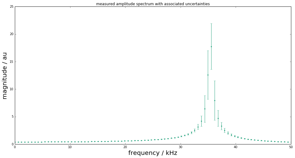
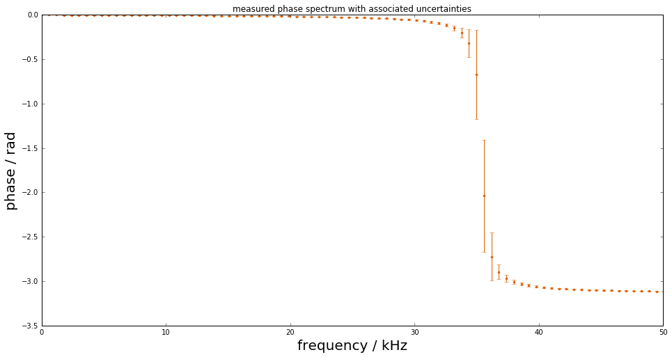
Assume information about a linear time-invariant (LTI) measurement system to be available in terms of its frequency response values \(H(j\omega)\) at a set of frequencies together with associated uncertainties:
figure(figsize=(16,8))
errorbar(f*1e-3, np.abs(Hf), uAbs, fmt=".", color=colors[0])
title("measured amplitude spectrum with associated uncertainties")
xlim(0,50)
xlabel("frequency / kHz",fontsize=20)
ylabel("magnitude / au",fontsize=20);
figure(figsize=(16,8))
errorbar(f*1e-3, np.angle(Hf), uPhas, fmt=".", color=colors[1])
title("measured phase spectrum with associated uncertainties")
xlim(0,50)
xlabel("frequency / kHz",fontsize=20)
ylabel("phase / rad",fontsize=20);
Simulated measurement
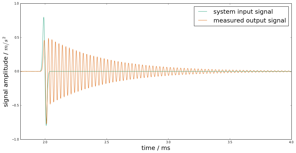
Measurements with this system are then modeled as a convolution of the system’s impulse response
with the input signal \(x(t)\), after an analogue-to-digital conversion producing the measured signal
# simulate input and output signals
time = np.arange(0, 4e-3 - Ts, Ts)
#x = shocklikeGaussian(time, t0 = 2e-3, sigma = 1e-5, m0=0.8)
m0 = 0.8; sigma = 1e-5; t0 = 2e-3
x = -m0*(time-t0)/sigma * np.exp(0.5)*np.exp(-(time-t0) ** 2 / (2 * sigma ** 2))
y = dsp.lfilter(b, a, x)
noise = 1e-3
yn = y + rst.randn(np.size(y)) * noise
figure(figsize=(16,8))
plot(time*1e3, x, label="system input signal", color=colors[0])
plot(time*1e3, yn,label="measured output signal", color=colors[1])
legend(fontsize=20)
xlim(1.8,4); ylim(-1,1)
xlabel("time / ms",fontsize=20)
ylabel(r"signal amplitude / $m/s^2$",fontsize=20);
Design of the deconvolution filter
The aim is to derive a digital filter with finite impulse response (FIR)
such that the filtered signal
is an estimate of the system’s input signal at the discrete time points.
Publication
Elster and Link “Uncertainty evaluation for dynamic measurements modelled by a linear time-invariant system” Metrologia, 2008
Vuerinckx R, Rolain Y, Schoukens J and Pintelon R “Design of stable IIR filters in the complex domain by automatic delay selection” IEEE Trans. Signal Process. 44 2339–44, 1996
Determine FIR filter coefficients such that
with a pre-defined time delay \(n_0\) to improve the fit quality (typically half the filter order).
Consider as least-squares problem
with - \(y\) real and imaginary parts of the reciprocal and phase shifted measured frequency response values - \(X\) the model matrix with entries \(e^{-j k \omega/Fs}\) - \(b\) the sought FIR filter coefficients - \(W\) a weighting matrix (usually derived from the uncertainties associated with the frequency response measurements
Filter coefficients and associated uncertainties are thus obtained as
# Calculation of FIR deconvolution filter and its assoc. unc.
N = 12; tau = N//2
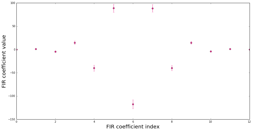
bF, UbF = LSFIR(H,N,tau,f,Fs,UH=UH)
Least-squares fit of an order 12 digital FIR filter to the
reciprocal of a frequency response given by 400 values
and propagation of associated uncertainties.
Final rms error = 1.545423e+01
figure(figsize=(16,8))
errorbar(range(N+1), bF, np.sqrt(np.diag(UbF)), fmt="o", color=colors[3])
xlabel("FIR coefficient index", fontsize=20)
ylabel("FIR coefficient value", fontsize=20);
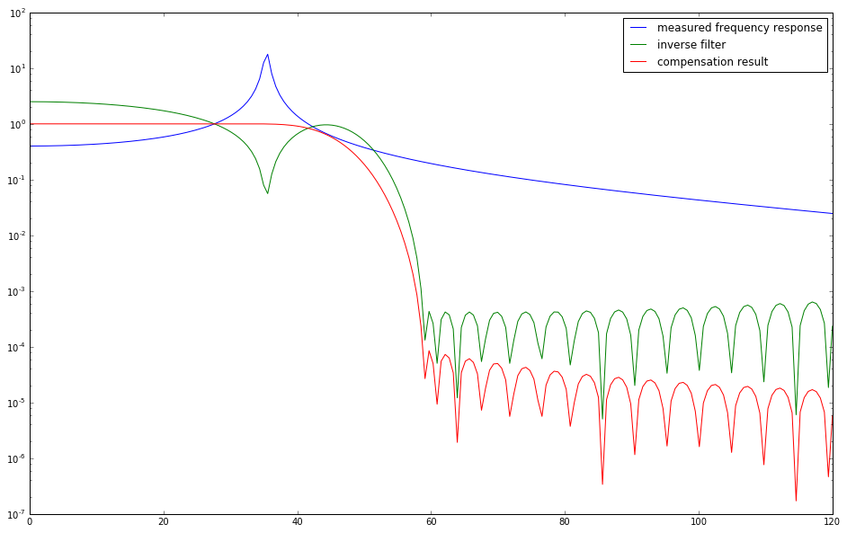
In order to render the ill-posed estimation problem stable, the FIR inverse filter is accompanied with an FIR low-pass filter.
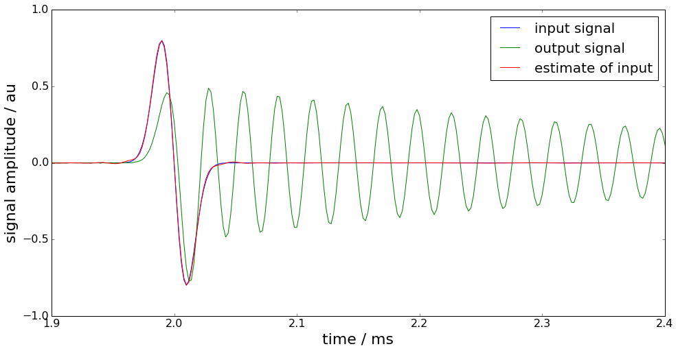
Application of the deconvolution filter for input estimation is then carried out as
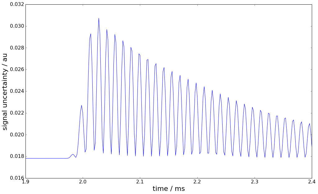
with point-wise associated uncertainties calculated as
fcut = f0+10e3; low_order = 100
blow, lshift = kaiser_lowpass(low_order, fcut, Fs)
shift = -tau - lshift
figure(figsize=(16,10))
HbF = dsp.freqz(bF,1,2*np.pi*f/Fs)[1]*dsp.freqz(blow,1,2*np.pi*f/Fs)[1]
semilogy(f*1e-3, np.abs(Hf), label="measured frequency response")
semilogy(f*1e-3, np.abs(HbF),label="inverse filter")
semilogy(f*1e-3, np.abs(Hf*HbF), label="compensation result")
legend();
xhat,Uxhat = FIRuncFilter(yn,noise,bF,UbF,shift,blow)
figure(figsize=(16,8))
plot(time*1e3,x, label='input signal')
plot(time*1e3,yn,label='output signal')
plot(time*1e3,xhat,label='estimate of input')
legend(fontsize=20)
xlabel('time / ms',fontsize=22)
ylabel('signal amplitude / au',fontsize=22)
tick_params(which="both",labelsize=16)
xlim(1.9,2.4); ylim(-1,1);
figure(figsize=(16,10))
plot(time*1e3,Uxhat)
xlabel('time / ms',fontsize=22)
ylabel('signal uncertainty / au',fontsize=22)
subplots_adjust(left=0.15,right=0.95)
tick_params(which='both', labelsize=16)
xlim(1.9,2.4);
Basic workflow in PyDynamic
Fit an FIR filter to the reciprocal of the measured frequency response
from PyDynamic.model_estimation.fit_filter import LSFIR
bF, UbF = LSFIR(H,N,tau,f,Fs,verbose=False,UH=UH)
with
Hthe measured frequency response valuesUHthe covariance (i.e. uncertainty) associated with real and imaginary parts ofHNthe filter ordertauthe filter delay in samplesfthe vector of frequencies at whichHis givenFsthe sampling frequency for the digital FIR filter
Propagate the uncertainty associated with the measurement noise and the FIR filter through the deconvolution process
xhat,Uxhat = FIRuncFilter(yn,noise,bF,UbF,shift,blow)
with
ynthe noisy measurementnoisethe std of the noiseshiftthe total delay of the FIR filter and the low-pass filterblowthe coefficients of the FIR low-pass filter