%pylab inline
colors = [[0.1,0.6,0.5], [0.9,0.2,0.5], [0.9,0.5,0.1]]
Populating the interactive namespace from numpy and matplotlib
Deconvolution in the frequency domain (DFT)
from PyDynamic.uncertainty.propagate_DFT import GUM_DFT,GUM_iDFT
from PyDynamic.uncertainty.propagate_DFT import DFT_deconv, AmpPhase2DFT
from PyDynamic.uncertainty.propagate_DFT import DFT_multiply
#%% reference data
ref_file = np.loadtxt("DFTdeconv reference_signal.dat")
time = ref_file[:,0]
ref_data = ref_file[:,1]
Ts = 2e-9
N = len(time)

#%% hydrophone calibration data
calib = np.loadtxt("DFTdeconv calibration.dat")
f = calib[:,0]
FR = calib[:,1]*np.exp(1j*calib[:,3])
Nf = 2*(len(f)-1)

uAmp = calib[:,2]
uPhas= calib[:,4]
UAP = np.r_[uAmp,uPhas*np.pi/180]**2

#%% measured hydrophone output signal
meas = np.loadtxt("DFTdeconv measured_signal.dat")
y = meas[:,1]
# assumed noise std
noise_std = 4e-4
Uy = noise_std**2
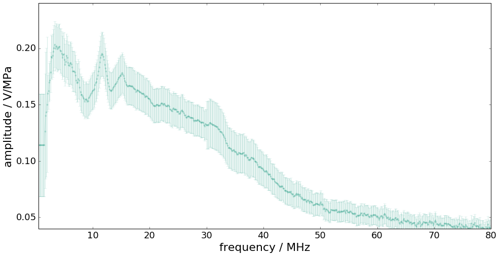
Consider knowledge about the measurement system is available in terms of its frequency response with uncertainties associated with amplitude and phase values.
figure(figsize=(16,8))
errorbar(f * 1e-6, abs(FR), 2 * sqrt(UAP[:len(UAP) // 2]), fmt= ".-", alpha=0.2, color=colors[0])
xlim(0.5, 80)
ylim(0.04, 0.24)
xlabel("frequency / MHz", fontsize=22); tick_params(which= "both", labelsize=18)
ylabel("amplitude / V/MPa", fontsize=22);
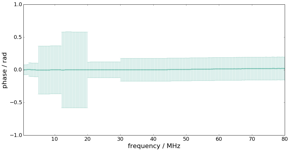
figure(figsize=(16,8))
errorbar(f * 1e-6, unwrap(angle(FR)) * pi / 180, 2 * UAP[len(UAP) // 2:], fmt= ".-", alpha=0.2, color=colors[0])
xlim(0.5, 80)
ylim(-0.2, 0.3)
xlabel("frequency / MHz", fontsize=22); tick_params(which= "both", labelsize=18)
ylim(-1,1)
ylabel("phase / rad", fontsize=22);
The measurand is the input signal \(\mathbf{x}=(x_1,\ldots,x_M)\) to the measurement system with corresponding measurement model given by
Input estimation is here to be considered in the Fourier domain.
The estimation model equation is thus given by
with - \(Y(f)\) the DFT of the measured system output signal - \(H_L(f)\) the frequency response of a low-pass filter
Estimation steps
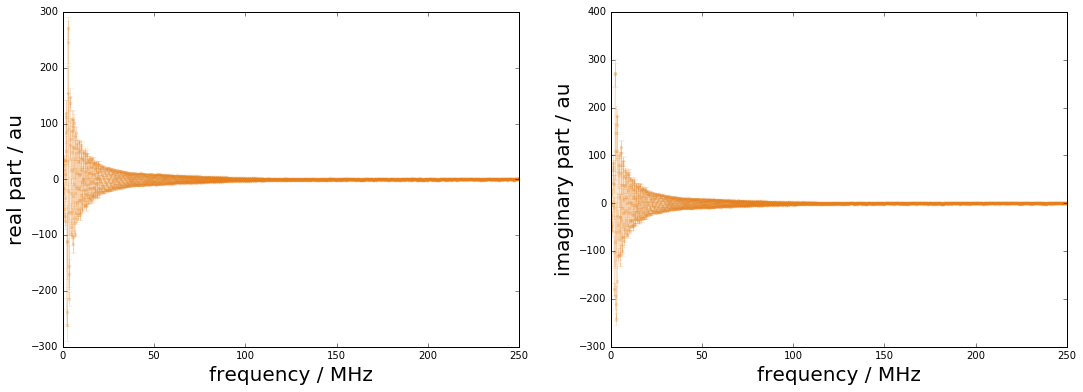
DFT of \(y\) and propagation of uncertainties to the frequency domain
Propagation of uncertainties associated with amplitude and phase of system to corr. real and imaginary parts
Division in the frequency domain and propagation of uncertainties
Multiplication with low-pass filter and propagation of uncertainties
Inverse DFT and propagation of uncertainties to the time domain
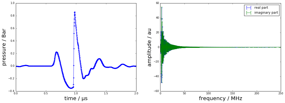
Propagation from time to frequency domain
With the DFT defined as
with \(\beta_n = 2\pi n /N\), the uncertainty associated with the DFT outcome represented in terms of real and imaginary parts, is given by
Y,UY = GUM_DFT(y,Uy,N=Nf)
figure(figsize=(18,6))
subplot(121)
errorbar(time*1e6, y, sqrt(Uy)*ones_like(y),fmt=".-")
xlabel("time / µs",fontsize=20); ylabel("pressure / Bar",fontsize=20)
subplot(122)
errorbar(f*1e-6, Y[:len(f)],sqrt(UY[:len(f)]),label="real part")
errorbar(f*1e-6, Y[len(f):],sqrt(UY[len(f):]),label="imaginary part")
legend()
xlabel("frequency / MHz",fontsize=20); ylabel("amplitude / au",fontsize=20);
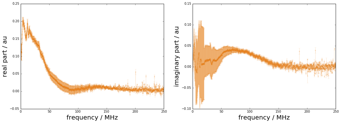
Uncertainties for measurement system w.r.t. real and imaginary parts
In practice, the frequency response of the measurement system is characterised in terms of its amplitude and phase values at a certain set of frequencies. GUM uncertainty evaluation, however, requires a representation by real and imaginary parts.
GUM uncertainty propagation
H, UH = AmpPhase2DFT(np.abs(FR),np.angle(FR),UAP)
Nf = len(f)
figure(figsize=(18,6))
subplot(121)
errorbar(f*1e-6, H[:Nf], sqrt(diag(UH[:Nf,:Nf])),fmt=".-",color=colors[2],alpha=0.2)
xlabel("frequency / MHz",fontsize=20); ylabel("real part / au",fontsize=20)
subplot(122)
errorbar(f*1e-6, H[Nf:],sqrt(diag(UH[Nf:,Nf:])),fmt=".-",color=colors[2],alpha=0.2)
xlabel("frequency / MHz",fontsize=20); ylabel("imaginary part / au",fontsize=20);
Deconvolution in the frequency domain
The deconvolution problem can be decomposed into a division by the system’s frequency response followed by a multiplication by a low-pass filter frequency response.
which in real and imaginary part becomes
Sensitivities for division part
Uncertainty blocks for multiplication part
# low-pass filter for deconvolution
def lowpass(f,fcut=80e6):
    return 1/(1+1j*f/fcut)**2

HLc = lowpass(f)
HL = np.r_[np.real(HLc), np.imag(HLc)]
XH,UXH = DFT_deconv(H,Y,UH,UY)

XH, UXH = DFT_multiply(XH, UXH, HL)
figure(figsize=(18,6))
subplot(121)
errorbar(f*1e-6, XH[:Nf], sqrt(diag(UXH[:Nf,:Nf])),fmt=".-",color=colors[2],alpha=0.2)
xlabel("frequency / MHz",fontsize=20); ylabel("real part / au",fontsize=20)
subplot(122)
errorbar(f*1e-6, XH[Nf:],sqrt(diag(UXH[Nf:,Nf:])),fmt=".-",color=colors[2],alpha=0.2)
xlabel("frequency / MHz",fontsize=20); ylabel("imaginary part / au",fontsize=20);
Propagation from frequency to time domain
The inverse DFT equation is given by
The sensitivities for the GUM propagation of uncertainties are then
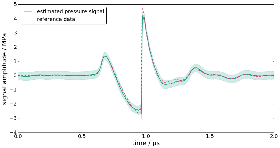
GUM uncertainty propagation for the inverse DFT
xh,Uxh = GUM_iDFT(XH,UXH,Nx=N)
ux = np.sqrt(np.diag(Uxh))

figure(figsize=(16,8))
plot(time*1e6,xh,label="estimated pressure signal",linewidth=2,color=colors[0])
plot(time * 1e6, ref_data, "--", label= "reference data", linewidth=2, color=colors[1])
fill_between(time * 1e6, xh + 2 * ux, xh - 2 * ux, alpha=0.2, color=colors[0])
xlabel("time / µs", fontsize=22)
ylabel("signal amplitude / MPa", fontsize=22)
tick_params(which= "major", labelsize=18)
legend(loc= "upper left", fontsize=18, fancybox=True)
xlim(0, 2);
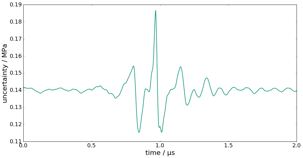
figure(figsize=(16,8))
plot(time * 1e6, ux, label= "uncertainty", linewidth=2, color=colors[0])
xlabel("time / µs", fontsize=22)
ylabel("uncertainty / MPa", fontsize=22)
tick_params(which= "major", labelsize=18)
xlim(0,2);
Summary of PyDynamic workflow for deconvolution in DFT domain
Y,UY = GUM_DFT(y,Uy,N=Nf)

H, UH = AmpPhase2DFT(A, P, UAP)

XH,UXH = DFT_deconv(H,Y,UH,UY)

XH, UXH = DFT_multiply(XH, UXH, HL)